PAC Theory and VC Dimension

Introduction to PAC Theory

In machine learning, we often grapple with a fundamental question: how well does our model, trained on limited data, perform on unseen examples? Probably Approximately Correct (PAC) learning theory provides a framework to address this question rigorously.

The Standard Setup

Let’s establish some notation and key concepts:

• $f_m$: The best function on our training set that minimizes empirical error ($\arg\min \hat{R}(f)$)

• $f^*$: The best function within our hypothesis space $\mathcal{H}$

• $f$: The exact objective function (the best in all possible space)

• True risk $R(f)$: What we ultimately want to minimize

• True risk ≈ Test error (as sample size approaches infinity)

• Excess risk = $R(f_m) - R^*$, which can be decomposed into:

  • Estimation error: $R(f_m) - R(f^*)$
  • Approximation error: $R(f^*) - R^*$
  • $R^*$: The Bayes risk, which represents the lowest possible risk achievable given the data distribution

For our analysis, let’s focus on understanding $R(f_m)$ and its relation to other error measures.

The Relationship Between Errors

The key relationships we need to understand are:

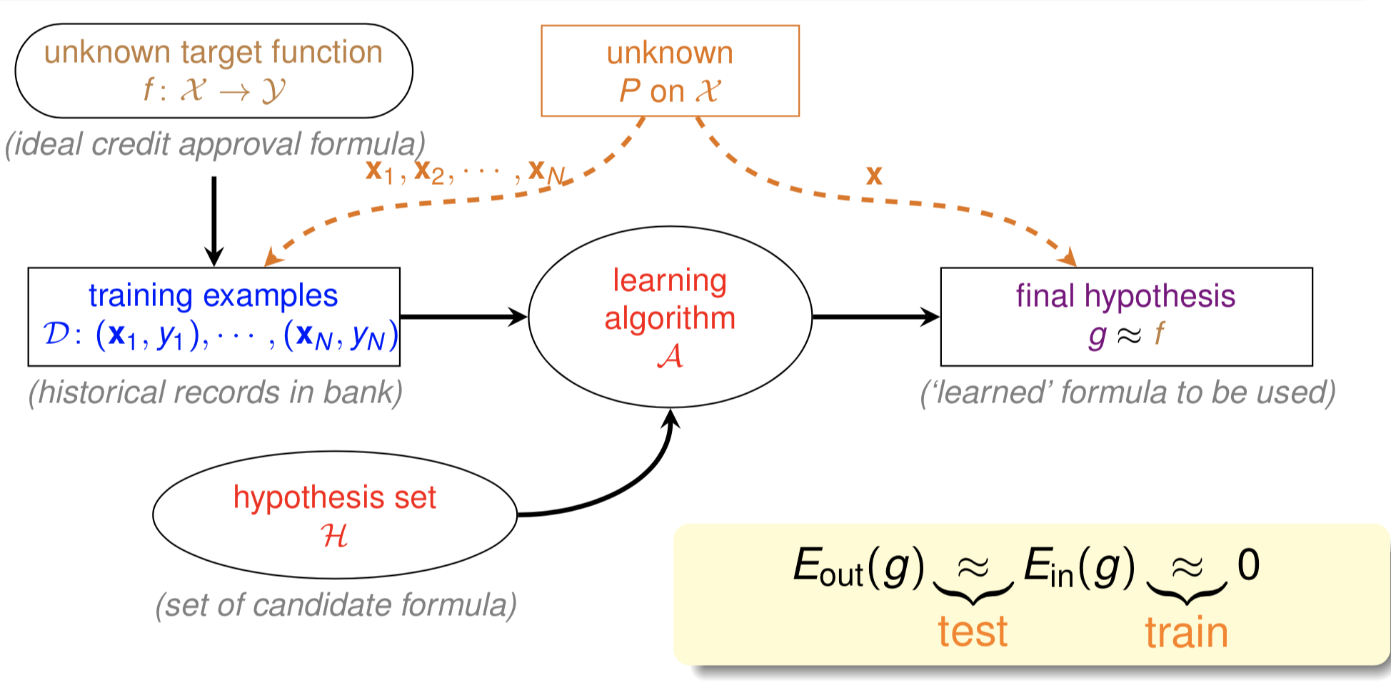
• $E_{out}(g) = R(f_m)$: The generalization error (estimation error or true risk)
• $E_{in}(g) = \hat{R}(f_m)$: The empirical error measured on training data
• $E_{out}(f) = R(f)$: The true risk of the ideal function

In the ideal scenario where $R(f) = 0$ and $fm$ approximates $f$ well, we want $R(f_m) \approx 0$. This leads to the desired chain of approximations: $0 = R(f) \approx R(f_m) \approx \hat{R}(f_m) \approx 0$

However, since we can’t access the full data distribution, we can’t calculate $R(f_m)$ directly. Instead, we need to bound it.

Bounding the True Risk

For a Single Function: Hoeffding’s Inequality

$\hat{R}(f)$ varies depending on our sample, while $R(f)$ is fixed. Using Hoeffding’s inequality:

$$P\left[|\nu - \mu| > \epsilon\right] \leq 2 \exp\left(-2\epsilon^2 N\right)$$

Where $\nu$ represents the sample expectation and $\mu$ is the true expectation. As our sample size $N$ increases, $\nu$ approaches $\mu$.

From Hoeffding’s inequality, we can see that as $N$ increases, the probability that the difference between $\nu$ and $\mu$ exceeds $\epsilon$ approaches zero. This means the sample expectation increasingly approximates the population expectation—they become “probably approximately correct.”

For any specific function, as $N$ grows: $\hat{R}(f_m) \approx R(f_m)$

$$\Pr\left( |E_{\text{in}}(h) - E_{\text{out}}(h)| > \epsilon \right) \leq 2 \exp\left(-2\epsilon^2 N\right)$$

For a Family of Functions: Uniform Deviation Bounds

Why we need our bound to simultaneously (or uniformly) hold over a family of functions?

Theorem: ERM’s estimation error is at most twice the uniform divergence

When dealing with multiple hypotheses, we must account for the fact that rare events become likely when tried many times. Consider this example: flipping a coin 5 times and getting all heads has a probability of 1/32. But if 100 people perform this experiment, the probability that at least one person gets all heads exceeds 0.95.

Using the union bound for a hypothesis space $\mathcal{H}$ with functions $f_1, f_2, \ldots, f_M$:

$$\forall g \in \mathcal{H}, \Pr\left( |E_{\text{in}}(g) - E_{\text{out}}(g)| > \epsilon \right) \leq 2M \exp\left(-2\epsilon^2 N\right)$$

This formula tells us that for any hypothesis $g$ in $\mathcal{H}$, the probability that the difference between $E_{in}(g)$ and $E_{out}(g)$ exceeds $\epsilon$ is bounded by $2M\exp(-2\epsilon^2 N)$. This bound heavily depends on both $M$ (the size of the hypothesis space) and $N$ (the sample size).

What Makes a Hypothesis Space Learnable?

A hypothesis space $\mathcal{H}$ is learnable if:

1. Algorithm $A$ can learn a function $f$ from $\mathcal{H}$ such that $\hat{R}(f) \approx 0$
2. In $\mathcal{H}$, $M$ is finite and $N$ is sufficiently large

When these conditions are met, the right side of our bound approaches 0, guaranteeing $R(f) \approx \hat{R}(f)$.

• In training: We minimize $\hat{R}(f)$ to find $f_m$
• In testing: We aim to minimize $R(f)$, which should be close to $\hat{R}(f)$

However, challenges arise when:

• $M$ is too small: It becomes difficult to find the exact $f$
• $M$ is too large: The right side doesn’t approach 0
• $M$ is infinite (which is common): This violates condition 2, making learning seemingly impossible

But wait—in most practical scenarios, $M$ is infinite. For instance, in a 2D space, we have infinitely many possible lines. Does this mean learning is impossible? This is where VC dimension comes in.

VC Dimension: Making the Infinite Manageable

The union bound can be loose because hypotheses in $\mathcal{H}$ aren’t completely independent—many can be categorized as essentially the same class.

This means $M$ can be rewritten as a finite “effective($M$)” depending on the sample:

$$\forall g \in \mathcal{H}, \Pr\left( |E_{\text{in}}(g) - E_{\text{out}}(g)| > \epsilon \right) \leq 2 \cdot \text{effective}(M) \exp\left(-2\epsilon^2 N\right)$$

Growth Function and Dichotomy

To understand the effective $M$, we introduce the concepts of dichotomy and growth function. Since we don’t want to depend on a specific data distribution $D$, we consider the maximum number of dichotomies across any $D$ in $\mathcal{H}$—this is the Growth Function.

The growth function represents the maximum possible number of labeling results that the hypothesis space $\mathcal{H}$ can assign to any $N$ samples. In simpler terms, it represents the number of meaningfully different hypotheses that can produce distinct results—the effective hypotheses.

A larger growth function indicates that $\mathcal{H}$ can express more classifiers, which leads to the question: can we substitute the effective($M$) with the Growth function?

Shattering and Break Points

When a hypothesis space $\mathcal{H}$ acting on a sample set $D$ of size $N$ produces $2^N$ dichotomies (Growth Function = $2^N$), we say $D$ is “shattered” by $\mathcal{H}$. In other words, if $\mathcal{H}$ can produce all possible dichotomies on a dataset, we say $\mathcal{H}$ can shatter that dataset.

The growth function helps us reduce $M$ from infinite to being bounded by $2^N$, but this is still too loose. We introduce the concept of a “break point”:

Starting from $N=1$ and gradually increasing, when we reach a value $k$ where the growth function becomes less than $2^N$, we say $k$ is the break point of the hypothesis space. In other words, for any dataset of size $N$ (where $N \geq k$), $\mathcal{H}$ cannot shatter it.

For example, if $\mathcal{H}$ consists of all lines in 2D space, the break point is 4.

With a break point, the upper bound becomes a polynomial $N^{k-1}$ rather than the exponential $2^N$. (Proof Here) ¹

$$m_H(N) \leq B(N, k) \leq \sum_{i=0}^{k-1} \binom{N}{i} \leq N^{k-1}$$

Then, the PAC bound with VC bound becomes (Proof Here) ²:

$$\forall g \in \mathcal{H}, \Pr\left( |E_{\text{in}}(g) - E_{\text{out}}(g)| > \epsilon \right) \leq 4 m_{\mathcal{H}}(2N) \exp\left(-\frac{1}{8} \epsilon^2 N\right)$$

While we can’t simply substitute effective $M$ with the Growth function, they are clearly related.

VC Dimension Defined

The VC dimension $d = k-1$ (where $k$ is the break point). The VC dimension indicates:

• There exists a dataset of size $d$ that can be shattered by hypothesis space $\mathcal{H}$
• $\mathcal{H}$ can at most shatter $d$ data points

It’s important to note that this doesn’t mean all datasets of size $d$ can be shattered by $\mathcal{H}$. For example, the hypothesis space of all lines in a 2D plane has a VC dimension of 3, but it cannot shatter three points lying on the same line. In fact, the VC dimension’s definition is independent of the specific data distribution.

With the growth function bounded by $N^d$, we get:

$$\forall g \in \mathcal{H}, \Pr\left( |E_{\text{in}}(g) - E_{\text{out}}(g)| > \epsilon \right) \leq 4(2N)^{V(\mathcal{H})} \exp\left(-\frac{1}{8} \epsilon^2 N\right)$$

Revisiting Learnability with VC Dimension

With these concepts in hand, we can redefine the second condition for learnability from “$M$ finite” to “VC dimension for $\mathcal{H}$ is finite.” The progression of our understanding has been: $M \rightarrow \text{Effective } M \rightarrow \text{Growth Function} \rightarrow \text{VC dimension}$

A larger VC dimension generally indicates a more complex model.

Importantly, the VC dimension is independent of:

• The learning algorithm
• The specific distribution of the dataset
• The objective function we solve

It depends only on the model and the hypothesis space. In practice, the VC dimension of a hypothesis space is approximately equal to the number of free parameters in the hypothesis.

The Tradeoff: Empirical Risk vs. True Risk

Finally, we can derive the relationship between $E_{in}(g)$ and $E_{out}(g)$, by inversely solve for

$$\epsilon = \sqrt{\frac{8}{N} \ln \left( \frac{4(2N)^{VC(H)}}{\delta} \right)}$$

it follows that there is a $1-\delta$ probability that something good will happen, and the good thing,

$$E_{in}(g) - \sqrt{\frac{8}{N} \ln \left( \frac{4(2N)^{VC(H)}}{\delta} \right)} \leq E_{out}(g) \leq E_{in}(g) + \sqrt{\frac{8}{N} \ln \left( \frac{4(2N)^{VC(H)}}{\delta} \right)}$$

This equation describes the relationship between $E_{in}(g)$ and $E_{out}(g)$. The square root term can be viewed as the model complexity $\Omega$—the more complex the model, the larger the gap between $E_{in}(g)$ and $E_{out}(g)$.

When we fix the sample size $N$, as the VC dimension increases, $E_{in}(g)$ continuously decreases while the complexity $\Omega$ increases. The rates of increase and decrease vary at different stages, so we need to find a suitable VC dimension that balances both factors to minimize $E_{out}(g)$.

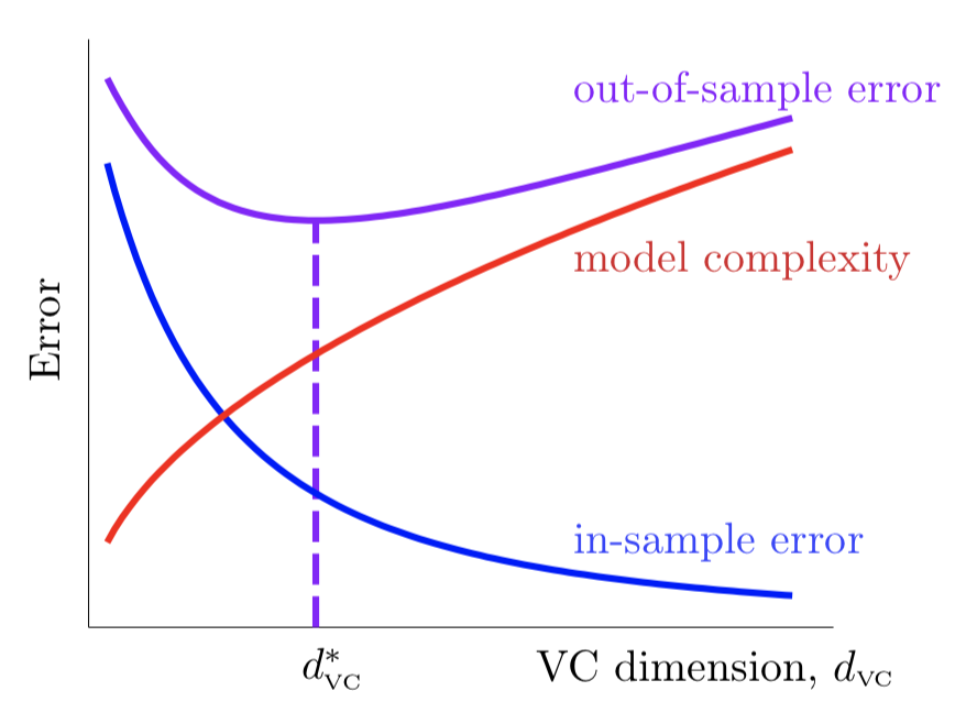
This relationship reveals the classic bias-variance tradeoff in machine learning: simpler models might have higher training error but generalize better, while more complex models can fit the training data perfectly but may perform poorly on unseen examples.

Conclusion

PAC theory and VC dimension provide a theoretical foundation for understanding when and why machine learning algorithms work. By quantifying the relationship between empirical and true risk, they help us navigate the fundamental tradeoff between model complexity and generalization performance.

Reference

1. 统计学习理论之VC维究竟是什么 | TangShusen
2. 深入理解 PAC 学习理论 | 阿平的自我修养